Analysing 3,000 Actuarial Tables

Mortality tables don’t really die: they just get rating adjustments and live on in surrender bases, legislation and all sorts of other places.

So having easy access to historic tables can be very useful. The Society of Actuaries generously provides an invaluable resource with over 3,000 mortality and other tables (to be precise, there are 3,012 tables at the time of writing) from around the world. Tables can be downloaded in Excel, CSV or XML formats.

Later, we'll share some code to help read individual tables in Python and R.

Whilst it's easy to access individual tables in Excel, it's not so easy to use Excel to get an overview of what's in the totality of the 3,000+ tables. That's really straightforward in Python or R so we’ve done some analysis of precisely what, where and when these tables relate to.

First of all, what sort of tables do we have?

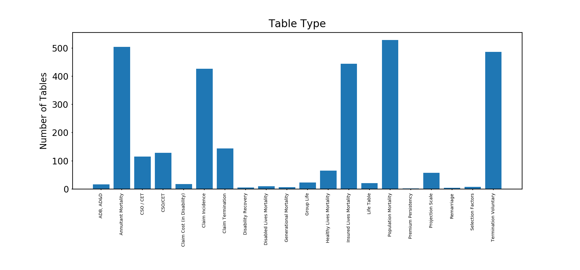
The majority of the tables are either mortality (Annuitant, Insured Lives or Population) or Health Insurance claim tables (Claim Incidence, and Claim Termination).

We can also look at country of origin:

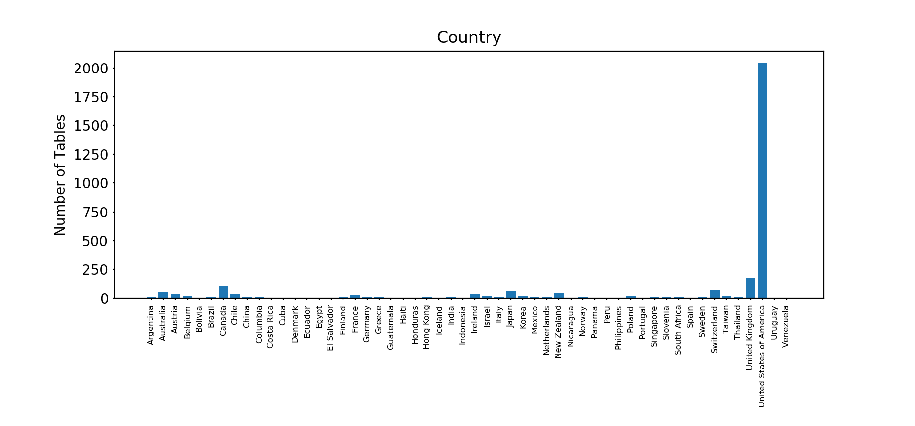
There are 54 unique nations. Unsurprisingly, the United States of America has the most tables, with 2,043, followed at a considerable distance by the United Kingdom with 174 and Canada with 105.

Next, what time period do these tables relate to? Here we’ve analysed the table description and found the most recent four digit year referred to in that description. Note that this doesn't pick up all the tables, as some have two digit years in their titles.

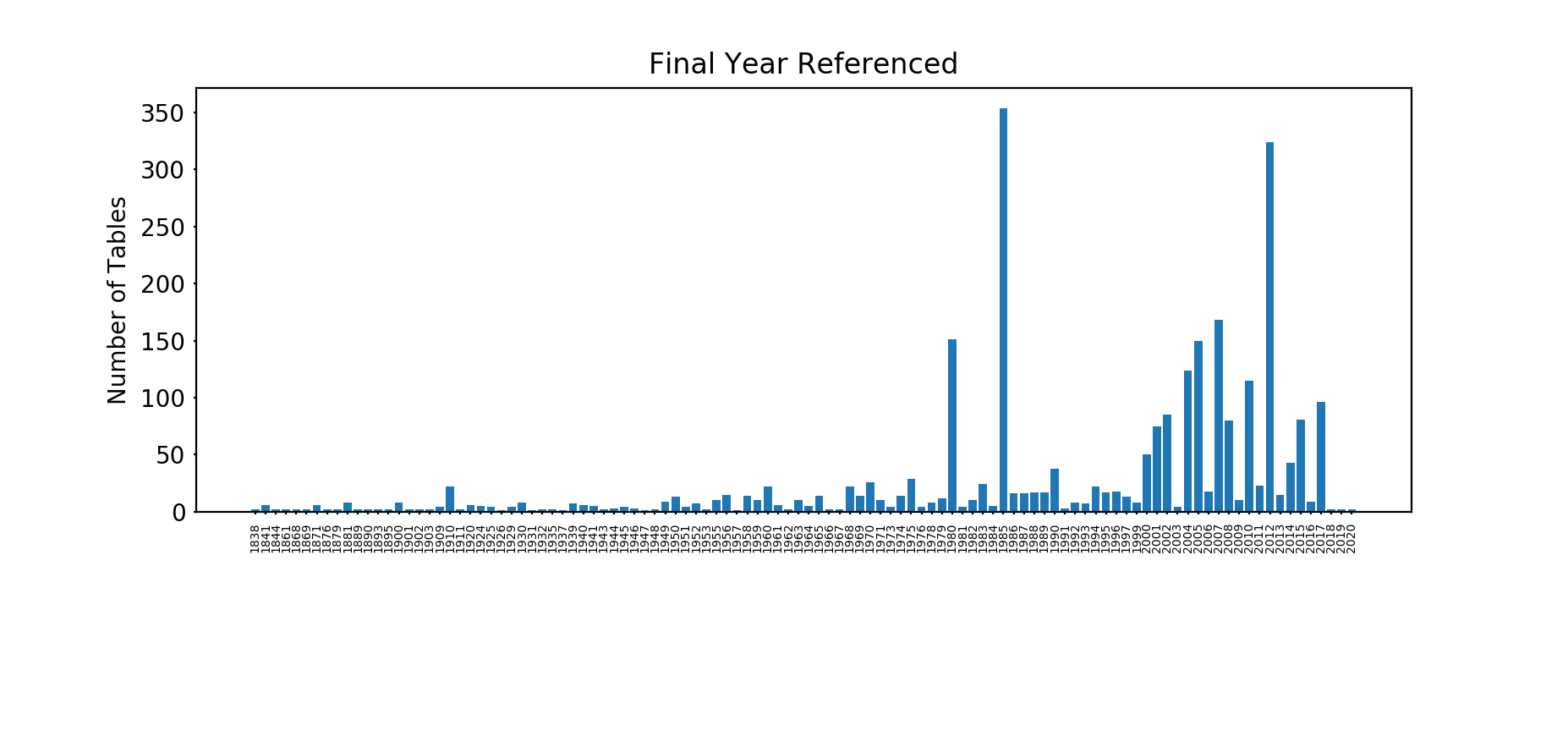
The oldest table is from 1838(!) - English Life Table No. 2, 1838-44 (whatever happened to English Life Table No. 1?) and the newest from 2020 (Mortality Improvement Scale MP-2020 from the SoA).

The peaks in 1985 and 2012 are interesting so let's have a closer look. The year 2012 has over 230 IDEC (Individual Disability Experience Committee) tables from the Society of Actuaries and over 70 Private Retirement Plan Mortality tables, again from the SoA. 1985 has around 280 CIDA (Commissioner's Individual Disability A) tables, again from the United States.

Finally, how many values are there in total in these tables? In total there are 1,914,817 numeric values across all 3,012 tables - or over 630 values per table. That's quite a lot of assumptions!

As promised, we've included some short code excerpts to help use these tables in practice. In each case we need the CSV file as downloaded from the Society of Actuaries website.

In Python, we just pass the file name to the read_table function and it returns pandas dataframes with the metadata and with the numerical data. The read_table function is just five lines of Python.

import pandas as pd

def read_table(table_file):
    table = pd.read_csv(table_file, header= None, encoding= 'unicode_escape')
    numeric_data = table[pd.to_numeric(table[0], errors='coerce').notnull()]
    meta_data = table[pd.to_numeric(table[0], errors='coerce').isnull()]
    return meta_data, numeric_data

def get_meta_tables(meta_data):
    mt = meta_data.copy().reset_index(drop=True)
    meta_tables = []
    while len(mt.index):
        table_row = mt[0].eq('Table # ').idxmax()
        rowcol_row = mt[0].eq('Row\Column').idxmax()
        meta_tables += [mt.iloc[table_row:rowcol_row + 1 , :].reset_index(drop=True).dropna(axis=1, how='all')]
        mt = mt.iloc[rowcol_row + 1: , :].reset_index(drop=True)
    return meta_tables

def get_data_tables(meta_tables, numeric):
    data_tables, index_start = [], 0
    for table in meta_tables:
        min_scale_value, max_scale_value, increment = int(table[1][8]), int(table[1][9]), int(table[1][10])
        table_length = 1
        if increment != 0:
            table_length = int(((max_scale_value - min_scale_value) + 1) / increment)
        index_end = index_start + table_length
        data_tables += [numeric[index_start:index_end].reset_index(drop=True).dropna(axis=1, how='all')]
        index_start = index_end
    return data_tables
    

One file can contain multiple tables. So, in addition, the get_meta_tables, get_data_tables functions attempt to parse the data returned by read_table into distinct tables, with the functions returning Python lists with the metadata and the numeric data for the tables respectively.

For R we have slightly simpler code - this time just reading the metadata and numeric data with no attempt to parse that data.

options(warn=-1)
mt <- read.csv(table_name, header=FALSE, stringsAsFactors=FALSE, encoding = "UTF-8")
numeric <- mt[!is.na(as.numeric(as.character(mt$V1))),]
meta <- mt[is.na(as.numeric(as.character(mt$V1))),]
row.names(numeric) <- NULL
row.names(meta) <- NULL
clean <- function(values) {return(iconv(values, "UTF-8", "UTF-8",sub=''))}
meta <- do.call(cbind.data.frame, lapply(meta, clean))
numeric <- do.call(cbind.data.frame, lapply(numeric, as.numeric))

We've tested this on a number of example tables but, of course, this code should be used at your own risk and you should validate the output before using for any production work.

Thanks again to the Society of Actuaries for this invaluable resource.

I hope you've found this interesting and useful. If so please share with your friends and colleagues. You can also follow us on twitter.

If you're working on an actuarial project using Python, R or any other data science tool or if you have any feedback then we'd love to hear from you! Do get in touch via the contact page.